Evolution of Energy Equipartition and the Boltzmann Distribution Law.

Introduction

This animation shows un-ambiguously that the evolution of the Boltzmann-like energy equipartition and final exponential energy distribution stems from the dynamics of collisions.

In this document, I first give the standard macroscopic Boltzmann treatment of the energy distribution of atoms of different mass. Then I describe just what and how the program computes its several different types of plots. Finally I show the mathematics of the velocity changes when two atoms of different mass and arbitrary velocities collide. Then I compute the average atom energies after collisions from those before collisions.

Standard Thermal Physics Treatment

The Boltzmann probability law for atom kinetic energy, E, is often written as:

$N (E) = N_{0} \exp (\frac{- E}{k T}) = N_{0} \exp (\frac{- m v^{2}}{2 k T})$

(1.1)

where N₀ is a normalization constant, m is the mass of the atom, k is Boltzmann's constant, v is the speed of the atom, and T is absolute temperature. It turns out, for the case of hard spheres and for real atoms, such as the noble gases that behave like hard spheres, that the E dependence of equation 1 is incorrect for both 1 and 3 dimensions[1] (see equation 26 with a=1/2 for 1 dimension and a=3/2 for 3 dimensions). For the important physical case of 3 dimensions the animations show that the appropriate equation for energy distribution is

$N (E) = N_{1} \sqrt{E} \exp (\frac{- E}{k T})$

(1.2)

as given in the above reference.

A more general expression for the range of dimensions d=1->3 is

$N (E) = N_{1} E^{\frac{d}{2} - 1} \exp (- \frac{E}{k T})$

(1.3)

For a derivation of this expression see a topic "Speed and Energy Distributions" in animation chapter "Gas Physics".

What the Animation Program Computes.

1. Energy Distribution N(E)

The program uses the results for velocity changes that are given in the next section to compute the kinetic energies of all of the atoms at each time increment. These energies are used to compute a bin number, b

$b = \frac{E}{E_{\max}} n_{b i n s}$

(1.4)

where E_max is several times larger than the average energy of all the atoms and n_bins is the number of energy bins that we use.

When an atom has bin number b, an integer array component, iE_b, is incremented by an the integer 1. After all of the atoms have been polled, iE contains the distribution of number of atoms Vs atom energy, N(E). But, since we use about 80 bins and we are limited to only about 1200 atoms, that would result, if N(E) is constant, in an average bin population of 15. The variance of 15 is about 4 and this would result in very erratic N(E). What we really want to know is the relative average occupancy of the energy bins. To obtain the final relative occupancy of the bins, it is acceptable to keep incrementing iE_b after each time interval. If we do this for a very large number of time increments, the initial transient changes of N(E) will be "averaged out". It is equivalent to taking many "snapshots" of the atomic energy distribution and averaging the results for each bin. Then what is plotted as a histogram is

$i E_{b} = \frac{1}{T} \sum_{t = 1}^{T} i E_{b, t}$

(1.5)

where t is the snapshot number and T is much greater than one.

The animation makes separate histograms for red and blue atoms. In addition, a least squares fit of an exponential function (the Boltzmann distribution) to the data in the histogram is made. The relative occupancy number (RON) equation is:

$N_{a} (E) = N_{0} \exp (- \frac{E}{< E >})$

(1.6)

where <E> is the average energy of the entire atom ensemble just as expected for a Boltzmann distribution. The animation shows beyond doubt that the RON equation has the same form and constants for red and blue atoms regardless of their masses, numbers and initial energies.

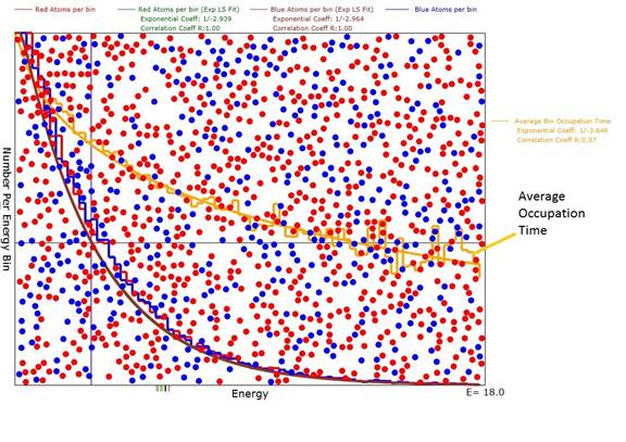
Figure 1: Diagram for d=2 dimensions of the animation after evolution was reasonably complete with an average energy <E>=3.0. Note that the green and purple exponential plots are a good fit to the red and blue atom numbers per bin histogram with correlation coefficients of 1.0. Also note that the exponential coefficients were very close to -1/3.0 as expected for a Boltzmann distribution.

2. The Average Energy Bin Occupancy Time τ(E)

The bin occupancy at low energy is expected to be longer than that at high energy and that asymmetry feeds into the exponential distribution of N(E). To compute the bin occupancy time, for each atom pair, c and d, that achieve the scatter condition, we record the time at which this occurs, t_0c and t_0d. Then, at the next time, t₁, that the scatter condition occurs, we take these differences t_1c-t_0c and t_1d-t_0d and increment a bin-based array by these numbers for each atom of the scattering pair. Since we want to have the average time between scatterings, we also increment a similar bin-based integer array by 1 for each of the pair. To get the average we use the fraction

$τ_{c, b} = \frac{1}{T_{c}} \sum_{t = 1}^{T_{c}} (t_{t + 1, c, b} - t_{t, c, b})$

(1.7)

$τ_{d, b} = \frac{1}{T_{d}} \sum_{t = 1}^{T_{d}} (t_{t + 1, d, b} - t_{t, d, b})$

(1.8)

When a least squares fit is done, this results in another exponential of the following form with respect to energy:

$τ (E) = τ_{0} \exp (- \frac{1}{2} \sqrt{\frac{E}{< E >}})$

(1.9)

where τ₀ is the average occupancy time at E=0 and <E> is the average energy of the entire ensemble of atoms.

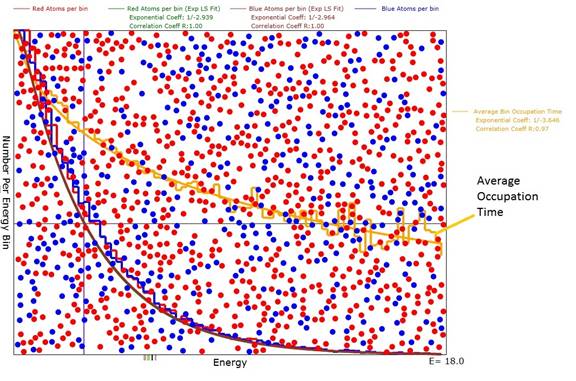
Figure 2: Diagram of the animation showing, in orange, the relative energy level occupation times Vs E. The smooth orange curve is a least squares fit to the occupation time. The coefficient is -1/(twice the square root of <E>) which in this case would be -1/3.5.

3. The Average Energy Change per Scatter

Although it is not included as a program option, I have separately computed the average energy change as a function of initial energies. The qualitative result is with initial energies above about 2<E> the energy change is negative while below initial energies of 2<E> the energy change is positive.

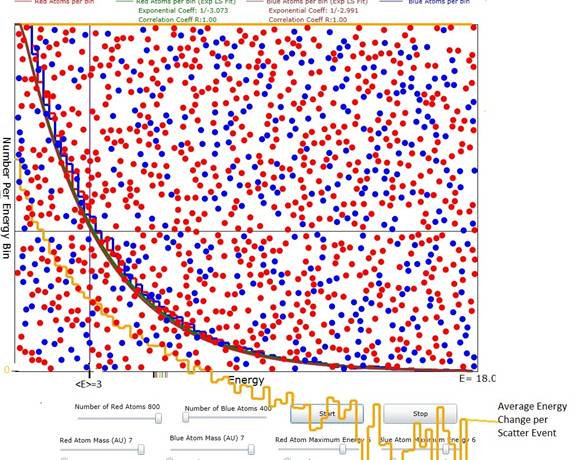
Figure 3: Diagram showing, in orange, the average energy change per scatter event. The zero of the energy change is the x axis of the plot as shown on the left. <E>=3 is clearly marked. At initial energy levels above about 2<E> the energy change is negative while at energy levels below about 2<E> the energy change is positive. The energy change could probably be fit to a gaussian of the same form as that for the average occupation time.

Mathematics of Hard Sphere Scattering

Atom-Atom Collisions of Different Mass and Velocity

Here we will consider spherical atoms which have the different masses, m₁ and m₂, and diameters, D₁ and D₂. The centers of the spheres will be labeled (x₁,y₁,z₁) and (x₂,y₂,z₂). Upon collision, the momentum transferred between the spheres will always be along the unit vector between their centers:

$u = \frac{[(x_{1} - x_{2}) \hat{x} + (y_{1} - y_{2}) \hat{y} + (z_{1} - z_{2}) \hat{z}]}{r_{12}}$

(1.10)

where

$r_{12} = \sqrt{{(x_{1} - x_{2})}^{2} + {(y_{1} - y_{2})}^{2} + {(z_{1} - z_{2})}^{2}}$

(1.11)

is the distance between centers. Since the animation is illustrated in only 2 dimensions, the collision analysis will assume a containing box that is large in the x and y dimensions but very thin in the z dimension. The following vector mathematics is correct for either 2 or three dimensions.

The expression for the final momenta in terms of the initial momenta is:

$m_{1} v_{1}^{'} + m_{2} v_{2}^{'} = m_{1} v_{1}^{} + m_{2} v_{2}^{}$

(1.12)

where the apostrophe on the left side of the equations indicates the final velocities. We know that the energies are conserved so

$\frac{m_{1} v_{1}^{' 2} + m_{2} v_{2}^{' 2}}{2} = \frac{m_{1} v_{1}^{2} + m_{1} v_{2}^{2}}{2}$

(1.13)

The directions of the change in momenta are along the vector of centers, u, and the values of the changes of momenta must be equal and opposite.

$m_{1} Δ v_{1} \equiv M δ v u = - m_{2} Δ v_{2}$

(1.14)

where M has units of mass and is still to be determined. Using equation 5 in equation 3:

$\begin{array}{l} m_{1} v_{1}^{'} = m_{1} v_{1}^{} + M δ v u \\ m_{2} v_{2}^{'} = m_{2} v_{2}^{} - M δ v u \end{array}$

(1.15)

Now we can use equation 6 in equation 4 to solve for the value of Mδv.

$\frac{(m_{1} v_{1}^{} + M δ v u) • (m_{1} v_{1}^{} + M δ v u)}{2 m_{1}} + \frac{(m_{2} v_{2}^{} - M δ v u) • (m_{2} v_{2}^{} - M δ v u)}{2 m_{2}} = \frac{m_{1} v_{1}^{2} + m_{2} v_{2}^{2}}{2}$

(1.16)

where the large dot stands for the dot product and equation 7 simplifies to:

$\begin{array}{l} \frac{(2 m_{1} M δ v u • v_{1}^{} + M^{2} δ v^{2})}{2 m_{1}} + \frac{(- 2 m_{2} M δ v u • v_{2}^{} + M^{2} δ v^{2})}{2 m_{2}} = 0 \\ M^{2} δ v^{2} (\frac{1}{m_{1}} + \frac{1}{m_{2}}) + 2 δ v M (u • v_{1}^{} - u • v_{2}^{}) = 0 \\ M δ v = \frac{2 m_{1} m_{2} u • (v_{2}^{} - v_{1}^{})}{m_{1} + m_{2}} \end{array}$

(1.17)

We can now make the identification:

$M = \frac{2 m_{1} m_{2}}{m_{1} + m_{2}}$

(1.18)

where M is known as the "reduced mass".

Equations (1.14) and (1.17) are a complete solution for the final momenta. The final velocities are computed by dividing both sides of equations (1.14) by their respective masses:

$\begin{array}{l} v_{1}^{'} = v_{1}^{} + \frac{2 m_{2}}{m_{1} + m_{2}} u • (v_{2}^{} - v_{1}^{}) u \\ v_{2}^{'} = v_{2}^{} - \frac{2 m_{1}}{m_{1} + m_{2}} u • (v_{2}^{} - v_{1}^{}) u \end{array}$

(1.19)

Suppose m₂>m₁. Then we see that the magnitude of the speed added to molecule 1 will be larger than the magnitude of the speed removed from molecule 2. We can easily see from equation 7, even though the averages of the dot products are zero, that, on average, the collision results in an increased kinetic energy for atom 1 and a decreased kinetic energy for molecule 2 because of the mass term in the denominators.

Summary of Results for Average Energies After Collision

After a collision with initial energies E₁₀ and E₂₀ we obtain the following results:

$\begin{array}{l} E_{1} = E_{10} + M δ v u • v_{1}^{} + \frac{{(M δ v)}^{2}}{2 m_{1}} = E_{10} + M [u • (v_{2}^{} - v_{1}^{})] (u • v_{1}^{}) + \frac{M^{2}}{2 m_{1}} [^{u • (v_{2}^{} - v_{1}^{})] 2} \\ E_{2} = E_{20} - M δ v u • v_{2}^{} + \frac{{(M δ v)}^{2}}{2 m_{2}} = E_{20} - M [u • (v_{2}^{} - v_{1}^{})] (u • v_{2}^{}) + \frac{M^{2}}{2 m_{2}} [^{u • (v_{2}^{} - v_{1}^{})] 2} \end{array}$

(1.20)

When the above result is averaged over all angles between u and v_i that actually lead to a collision i.e. u.(v₂-v₁)<0 we obtain:

$< E_{1} > = E_{10} - \frac{M v_{1}^{2}}{2} + \frac{M^{2}}{4 m_{1}} (v_{2}^{2} + v_{1}^{2}) = E_{10} - M (\frac{E_{10}}{m_{1}}) + \frac{M^{2}}{2 m_{1}} (\frac{E_{10}}{m_{1}} + \frac{E_{20}}{m_{2}})$

(1.21)

$< E_{2} > = E_{20} - \frac{M v_{2}^{2}}{2} + \frac{M^{2}}{4 m_{2}} (v_{2}^{2} + v_{1}^{2}) = E_{20} - M (\frac{E_{20}}{m_{2}}) + \frac{M^{2}}{2 m_{2}} (\frac{E_{10}}{m_{1}} + \frac{E_{20}}{m_{2}})$

(1.22)

Summary of Average Energy Results for m₁=m₂=m

When m₁=m₂=m so that M=m the results for average E, <E> , are easily seen from equations (1.21) and (1.22) to be:

$< E_{1} > = \frac{E_{10} + E_{20}}{2} = < E_{2} >$

(1.23)

With a little more difficulty the results for the variances of E, <ΔΕ>, are given by the following equations:

$\begin{array}{l} < Δ E_{1} > = \frac{E_{10} + E_{20}}{4} = < Δ E_{2} > w h e n E_{10} = E_{20} \\ < Δ E_{1} > = \sqrt{2} \frac{E_{10} + E_{20}}{4} = < Δ E_{2} > w h e n E_{10} = 0 o r E_{20} = 0 \end{array}$

(1.24)

Discussion of Scattering for Equal Mass Atoms.

So, what really happens when the masses are equal, is that the energies redistribute themselves into a gaussian-like pattern with the gaussian width greater when the energy differences are greater. Of course, the minimum outcome for any energy is always zero, so the distribution tends to become biased toward its E=0 end.

If we start with mono-energetic atoms, E₀, so that E_total=2E₀, then the first variance will always be 0.250E₀. A fraction of these scattered atoms will have energy 2E₀ and an exactly equal fraction will have zero energy. The next scattering, when with atoms with energies E₀, can result in energies from zero energy up to 3E₀. When the next scattering is between 2 atoms that have energy of 2E₀ the final energy can be as large as 4E₀ but that is a very unlikely event. Of course, since neither is moving, atoms with zero energy don't scatter with other atoms of zero energy so these latter remain at zero energy. In fact the number of scatterings per second depends on the energy of the atoms, so this makes all the lower energy atoms less likely to scatter with similar low energy atoms.

We could write the following approximate differential equation for the rate of scattering of atoms

$\frac{d N}{d t} = n σ v_{r} \propto n σ \sqrt{\frac{2 E_{1}}{m_{1}} + \frac{2 E_{2}}{m_{2}}}$

(1.25)

where n is the atom density, v_r is some average relative speed, and σ is the collision cross section. Thus the rate of change of energies via scattering depends on the sum of the velocities of the two atoms involved. This is one of the mechanisms that I think would cancel out the usual tendency for the atoms to form a symmetric gaussian distribution centered at the average energy. The other mechanism is that, while any energy higher than the average energy is possible, the minimum energy is always zero so a lot of atoms tend to accumulate near the zero end of the number Vs energy distribution.

We can also say that there are few high energy atoms because they scatter quite often so that they usually get their energies degraded by scattering with lower energy atoms and become "thermalized".